
Table of Contents
Chapter 1: Weibull Does as Data Is ....................................................9
Chapter 2: The Problems Weibull Can Address ...............................17
Chapter 3: Population, Data & the Linear Conjecture .....................30
Chapter 4: Routine Median Percent Computation ............................62
Chapter 5: Characterizing Weibull Populations ................................71
Chapter 6: Weibull Equations and Analysis Methods .....................103
Chapter 7: Weibull Analysis - What Can Go Wrong? .....................128
Chapter 8: Weibull Risk Analysis, Present & Future ......................148
Chapter 9: Weibull vs. R&M ...........................................................172
Chapter 10: Three Parameter Weibull Equations ............................190
Chapter 11: Computer Programs & Weibull Analysis .....................201
Chapter 12: Weibull Analysis in Retrospect ....................................214
Appendix A: Tables of Median Percent ...........................................218
Appendix B: Weibull Plot Analysis Tables ......................................219
Appendix C: Review of PDFs and CDFs .........................................222
Appendix D: Binomial Equation & Median Percent Calculation ... 233
Appendix E: Justifying the Linear Conjecture .................................240
Appendix F: Data Point Count & Weibull Accuracy .......................250
Appendix G: List of Conducted Weibull Studies .............................258
Appendix H: Useful Equations and Derivations ..............................260
Appendix J: Small Sample Analysis Examples ................................262
Appendix K: Rank Order Adjustment Theory ..................................274
Appendix L: The Use of 3 Parameter Weibulls ................................279
Appendix M: Sources of Statistical Data ..........................................285
Appendix N: Data Use Authorizations ..............................................287
Appendix O: Bibliography ................................................................292
A rather odd name for a chapter and a brief explanation is needed. John Berner at Applications Research commented, "What sets Weibull analysis apart is its unique ability to fit the Weibull equation through data-points as opposed to shoe-horning an unwilling equation onto the data." After consideration, I realized John is right and my task is to explain what he meant.
A summary level Weibull analysis follows showing what "fitting the Weibull equation through data-points" means. This will be contrasted to a Gaussian Bell Curve analysis which
Chapter 1 presents broad concepts. Only a general understanding is needed before moving on to following chapters which explain the "hows and whys" of doing actual analysis.
Historical Height of Tsunami Waves:

Figure 1-1: The Great 1928 Japan Tsunami (1)
Weibull analysis of Tsunamis was chosen to contrast Weibull success in fitting the equation through data-points versus Gaussian failure to describe data (2).
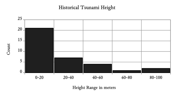
Figure 1-2: Tsunami Height Histogram

Figure 1-3: Weibull Plot of Tsunami Wave Heights
Figure 1-3 is a Weibull plot of data, based on pseudo x,y values explained in later chapters.
The Weibull Plot is very useful; but, statisticians usually create a Probability Density Function (PDF) as shown below from Weibull Plot information. Such PDF graphs represent percent of population as area. (PDFs are fully explained later and also in Appendix C.)
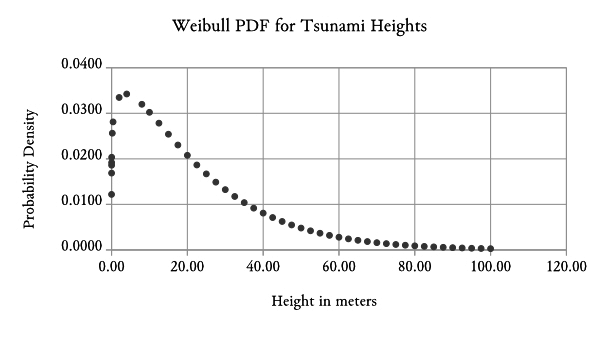
Figure 1-4: Weibull Tsunami PDF
PDF graphs are effectively histograms similar to Figure 1-2; but adapted to the continuous x number line in contrast to histograms, which divide the x axis into various "range buckets". Because PDF Figure 1-4 is effectively a histogram, its shape should be similar to Figure 1-2. The reader should compare the two figures and confirm the following:
While minor differences are evident between histogram and Weibull PDF, both the x range and general shape are very similar. We next examine a Gaussian (or Bell Curve) analysis performed on the same data, create its PDF and make comparisons. It will be shown that the Gaussian (or Bell Curve) PDF grossly misrepresents the histogram.
When a data-set is analyzed by a Gaussian Distribution, a 3 step process forces the data to "give up" a mean μ and a variance σ^2 which fully define the Bell curve PDF Figure 1-5.
By using values of mean and variance computed above, an exact Gaussian Equation is written which (hopefully) describes the data. Spreadsheet use of the Gaussian equation creates PDF Figure 1-5.
Step 2 and 3 of the Gaussian Analysis were performed by spreadsheet resulting in: Mean μ=22.34 and variance σ^2 = 530.84. Taking the square root the more commonly used standard deviation σ=23.04 is computed. For Gaussian analysis, there is no Weibull Plot equivalent, and hence no forcing of equation through data-points. The following Gaussian PDF is graphed based on mean and variance.

Figure 1-5: Gaussian PDF
As previously discussed, PDF graph (Figure 1-5) is really a histogram adapted to a continuous x number line. As such, the shape of the PDF should strongly resemble histogram Figure 1-2, BUT IT DOES NOT! Please compare Figures 1-2 and 1-5:
In general, the shape of the Gaussian Histogram is "just plain wrong."
A Weibull description of Tsunami data does a reasonable job of describing the trends we see in the data but a Gaussian description does not. While the Gaussian description computes a true average height, it incorrectly indicates 20% of Tsunamis have negative height (i.e. are depressions rather than humps in the ocean). The Gaussian PDF also incorrectly indicates a wave of just over 20 meters is the most frequent; but, Figure 1-2 shows that small waves are the most prevalent. Stated bluntly, the Gaussian "Bell Curve" misrepresents the actual distribution of wave heights.
For describing tsunami waves, Weibull analysis is an appropriate method of characterization and Gaussian analysis is not. The success of Weibull for this and many other problems results from the Weiubll Plot which is unique in its attempt to force the Weibull equation through the data-points. A successful attempt at forcing equation through data-points is evidenced by tightly fit data-points about the straight Weibull line (Figure 1-3). Problems do exist where even Weibull cannot describe the data; but, in such cases, the Weibull Plot provides clear evidence of its inability. By contrast, a failed Gaussian analysis provides no clear signal of its failure; thus encouraging the analyst to assume "all is well."
When Weibull is compared to other statistical distributions (Gaussian, Log Normal etc.), Webiull exhibits a greater ability to twist and turn in conformance to data points. As a result, Weibull has greater likelihood of successfully describing a data-set. Figure 1-6 below illustrates the various shapes Weibull can take. Changes to the Eta parameter, can stretch the shape horizontally if needed.

Figure 1-6: Weibull Shape Flexibility
It is possible to create a data-set that exactly represents a Gauss Distribution, or a Log Normal distribution or a decreasing Exponential Distribution. When tested against such data-sets, Weibull has been proven capable of describing all three.
When Gaussian analysis is used to analyze a data-set of 25 or more points, it is common to create a histogram to make sure that the Gauss PDF is similar in shape to actual data. Unfortunately, when small data-sets (e.g. 9 data-points) are analyzed, a convincing histogram cannot be made and other methods (e.g. Filliben's Probability Plot Coefficient Test for Normality) are needed. By contrast, the Weibull Plot provides clear evidence of either success or failure.
Finally, Weibull Analysis has been proven to successfully describe a wide range of phenomena. A few of the populations that have been characterized by a Weibull distribution include:
Footnotes:
Copyright 2022 by Paul F. Watson
All Rights Reserved
Updated 25 March 2022